Non-linear Least Squares
Introduction
Ceres can solve bounds constrained robustified non-linear least squares problems of the form
Problems of this form comes up in a broad range of areas across science and engineering - from fitting curves in statistics, to constructing 3D models from photographs in computer vision.
In this chapter we will learn how to solve (1) using Ceres Solver. Full working code for all the examples described in this chapter and more can be found in the examples directory.
The expression
\(\rho_i\left(\left\|f_i\left(x_{i_1},...,x_{i_k}\right)\right\|^2\right)\)
is known as a ResidualBlock, where \(f_i(\cdot)\) is a
CostFunction that depends on the parameter blocks
\(\left[x_{i_1},... , x_{i_k}\right]\). In most optimization
problems small groups of scalars occur together. For example the three
components of a translation vector and the four components of the
quaternion that define the pose of a camera. We refer to such a group
of small scalars as a ParameterBlock. Of course a
ParameterBlock can just be a single parameter. \(l_j\) and
\(u_j\) are bounds on the parameter block \(x_j\).
\(\rho_i\) is a LossFunction. A LossFunction is
a scalar function that is used to reduce the influence of outliers on
the solution of non-linear least squares problems.
As a special case, when \(\rho_i(x) = x\), i.e., the identity function, and \(l_j = -\infty\) and \(u_j = \infty\) we get the more familiar non-linear least squares problem.
Hello World!
To get started, consider the problem of finding the minimum of the function
This is a trivial problem, whose minimum is located at \(x = 10\), but it is a good place to start to illustrate the basics of solving a problem with Ceres [1].
The first step is to write a functor that will evaluate this the function \(f(x) = 10 - x\):
struct CostFunctor {
   template <typename T>
   bool operator()(const T* const x, T* residual) const {
     residual[0] = 10.0 - x[0];
     return true;
   }
};
The important thing to note here is that operator() is a templated
method, which assumes that all its inputs and outputs are of some type
T. The use of templating here allows Ceres to call
CostFunctor::operator<T>(), with T=double when just the value
of the residual is needed, and with a special type T=Jet when the
Jacobians are needed. In Derivatives we will discuss the
various ways of supplying derivatives to Ceres in more detail.
Once we have a way of computing the residual function, it is now time to construct a non-linear least squares problem using it and have Ceres solve it.
int main(int argc, char** argv) {
  google::InitGoogleLogging(argv[0]);

  // The variable to solve for with its initial value.
  double initial_x = 5.0;
  double x = initial_x;

  // Build the problem.
  Problem problem;

  // Set up the only cost function (also known as residual). This uses
  // auto-differentiation to obtain the derivative (jacobian).
  CostFunction* cost_function =
      new AutoDiffCostFunction<CostFunctor, 1, 1>();
  problem.AddResidualBlock(cost_function, nullptr, &x);

  // Run the solver!
  Solver::Options options;
  options.linear_solver_type = ceres::DENSE_QR;
  options.minimizer_progress_to_stdout = true;
  Solver::Summary summary;
  Solve(options, &problem, &summary);

  std::cout << summary.BriefReport() << "\n";
  std::cout << "x : " << initial_x
            << " -> " << x << "\n";
  return 0;
}
AutoDiffCostFunction takes a CostFunctor as input,
automatically differentiates it and gives it a CostFunction
interface.
Compiling and running examples/helloworld.cc gives us
iter      cost      cost_change  |gradient|   |step|    tr_ratio  tr_radius  ls_iter  iter_time  total_time
   0  4.512500e+01    0.00e+00    9.50e+00   0.00e+00   0.00e+00  1.00e+04       0    5.33e-04    3.46e-03
   1  4.511598e-07    4.51e+01    9.50e-04   9.50e+00   1.00e+00  3.00e+04       1    5.00e-04    4.05e-03
   2  5.012552e-16    4.51e-07    3.17e-08   9.50e-04   1.00e+00  9.00e+04       1    1.60e-05    4.09e-03
Ceres Solver Report: Iterations: 2, Initial cost: 4.512500e+01, Final cost: 5.012552e-16, Termination: CONVERGENCE
x : 0.5 -> 10
Starting from a \(x=5\), the solver in two iterations goes to 10 [2]. The careful reader will note that this is a linear problem and one linear solve should be enough to get the optimal value. The default configuration of the solver is aimed at non-linear problems, and for reasons of simplicity we did not change it in this example. It is indeed possible to obtain the solution to this problem using Ceres in one iteration. Also note that the solver did get very close to the optimal function value of 0 in the very first iteration. We will discuss these issues in greater detail when we talk about convergence and parameter settings for Ceres.
Footnotes
Derivatives
Ceres Solver like most optimization packages, depends on being able to evaluate the value and the derivatives of each term in the objective function at arbitrary parameter values. Doing so correctly and efficiently is essential to getting good results. Ceres Solver provides a number of ways of doing so. You have already seen one of them in action – Automatic Differentiation in examples/helloworld.cc
We now consider the other two possibilities. Analytic and numeric derivatives.
Numeric Derivatives
In some cases, its not possible to define a templated cost functor,
for example when the evaluation of the residual involves a call to a
library function that you do not have control over. In such a
situation, numerical differentiation can be used. The user defines a
functor which computes the residual value and construct a
NumericDiffCostFunction using it. e.g., for \(f(x) = 10 - x\)
the corresponding functor would be
struct NumericDiffCostFunctor {
  bool operator()(const double* const x, double* residual) const {
    residual[0] = 10.0 - x[0];
    return true;
  }
};
Which is added to the Problem as:
CostFunction* cost_function =
  new NumericDiffCostFunction<NumericDiffCostFunctor, ceres::CENTRAL, 1, 1>();
problem.AddResidualBlock(cost_function, nullptr, &x);
Notice the parallel from when we were using automatic differentiation
CostFunction* cost_function =
    new AutoDiffCostFunction<CostFunctor, 1, 1>();
problem.AddResidualBlock(cost_function, nullptr, &x);
The construction looks almost identical to the one used for automatic
differentiation, except for an extra template parameter that indicates
the kind of finite differencing scheme to be used for computing the
numerical derivatives [3]. For more details see the documentation
for NumericDiffCostFunction.
Generally speaking we recommend automatic differentiation instead of numeric differentiation. The use of C++ templates makes automatic differentiation efficient, whereas numeric differentiation is expensive, prone to numeric errors, and leads to slower convergence.
Analytic Derivatives
In some cases, using automatic differentiation is not possible. For example, it may be the case that it is more efficient to compute the derivatives in closed form instead of relying on the chain rule used by the automatic differentiation code.
In such cases, it is possible to supply your own residual and jacobian
computation code. To do this, define a subclass of
CostFunction or SizedCostFunction if you know the
sizes of the parameters and residuals at compile time. Here for
example is SimpleCostFunction that implements \(f(x) = 10 -
x\).
class QuadraticCostFunction : public ceres::SizedCostFunction<1, 1> {
 public:
  virtual ~QuadraticCostFunction() {}
  virtual bool Evaluate(double const* const* parameters,
                        double* residuals,
                        double** jacobians) const {
    const double x = parameters[0][0];
    residuals[0] = 10 - x;

    // Compute the Jacobian if asked for.
    if (jacobians != nullptr && jacobians[0] != nullptr) {
      jacobians[0][0] = -1;
    }
    return true;
  }
};
SimpleCostFunction::Evaluate is provided with an input array of
parameters, an output array residuals for residuals and an
output array jacobians for Jacobians. The jacobians array is
optional, Evaluate is expected to check when it is non-null, and
if it is the case then fill it with the values of the derivative of
the residual function. In this case since the residual function is
linear, the Jacobian is constant [4] .
As can be seen from the above code fragments, implementing
CostFunction objects is a bit tedious. We recommend that
unless you have a good reason to manage the jacobian computation
yourself, you use AutoDiffCostFunction or
NumericDiffCostFunction to construct your residual blocks.
More About Derivatives
Computing derivatives is by far the most complicated part of using
Ceres, and depending on the circumstance the user may need more
sophisticated ways of computing derivatives. This section just
scratches the surface of how derivatives can be supplied to
Ceres. Once you are comfortable with using
NumericDiffCostFunction and AutoDiffCostFunction we
recommend taking a look at DynamicAutoDiffCostFunction,
CostFunctionToFunctor, NumericDiffFunctor and
ConditionedCostFunction for more advanced ways of
constructing and computing cost functions.
Footnotes
Powell’s Function
Consider now a slightly more complicated example – the minimization of Powell’s function. Let \(x = \left[x_1, x_2, x_3, x_4 \right]\) and
\(F(x)\) is a function of four parameters, has four residuals and we wish to find \(x\) such that \(\frac{1}{2}\|F(x)\|^2\) is minimized.
Again, the first step is to define functors that evaluate of the terms in the objective functor. Here is the code for evaluating \(f_4(x_1, x_4)\):
struct F4 {
  template <typename T>
  bool operator()(const T* const x1, const T* const x4, T* residual) const {
    residual[0] = sqrt(10.0) * (x1[0] - x4[0]) * (x1[0] - x4[0]);
    return true;
  }
};
Similarly, we can define classes F1, F2 and F3 to evaluate
\(f_1(x_1, x_2)\), \(f_2(x_3, x_4)\) and \(f_3(x_2, x_3)\)
respectively. Using these, the problem can be constructed as follows:
double x1 =  3.0; double x2 = -1.0; double x3 =  0.0; double x4 = 1.0;

Problem problem;

// Add residual terms to the problem using the autodiff
// wrapper to get the derivatives automatically.
problem.AddResidualBlock(
  new AutoDiffCostFunction<F1, 1, 1, 1>(), nullptr, &x1, &x2);
problem.AddResidualBlock(
  new AutoDiffCostFunction<F2, 1, 1, 1>(), nullptr, &x3, &x4);
problem.AddResidualBlock(
  new AutoDiffCostFunction<F3, 1, 1, 1>(), nullptr, &x2, &x3);
problem.AddResidualBlock(
  new AutoDiffCostFunction<F4, 1, 1, 1>(), nullptr, &x1, &x4);
Note that each ResidualBlock only depends on the two parameters
that the corresponding residual object depends on and not on all four
parameters. Compiling and running examples/powell.cc
gives us:
Initial x1 = 3, x2 = -1, x3 = 0, x4 = 1
iter      cost      cost_change  |gradient|   |step|    tr_ratio  tr_radius  ls_iter  iter_time  total_time
   0  1.075000e+02    0.00e+00    1.55e+02   0.00e+00   0.00e+00  1.00e+04        0    2.91e-05    3.40e-04
   1  5.036190e+00    1.02e+02    2.00e+01   0.00e+00   9.53e-01  3.00e+04        1    4.98e-05    3.99e-04
   2  3.148168e-01    4.72e+00    2.50e+00   6.23e-01   9.37e-01  9.00e+04        1    2.15e-06    4.06e-04
   3  1.967760e-02    2.95e-01    3.13e-01   3.08e-01   9.37e-01  2.70e+05        1    9.54e-07    4.10e-04
   4  1.229900e-03    1.84e-02    3.91e-02   1.54e-01   9.37e-01  8.10e+05        1    1.91e-06    4.14e-04
   5  7.687123e-05    1.15e-03    4.89e-03   7.69e-02   9.37e-01  2.43e+06        1    1.91e-06    4.18e-04
   6  4.804625e-06    7.21e-05    6.11e-04   3.85e-02   9.37e-01  7.29e+06        1    1.19e-06    4.21e-04
   7  3.003028e-07    4.50e-06    7.64e-05   1.92e-02   9.37e-01  2.19e+07        1    1.91e-06    4.25e-04
   8  1.877006e-08    2.82e-07    9.54e-06   9.62e-03   9.37e-01  6.56e+07        1    9.54e-07    4.28e-04
   9  1.173223e-09    1.76e-08    1.19e-06   4.81e-03   9.37e-01  1.97e+08        1    9.54e-07    4.32e-04
  10  7.333425e-11    1.10e-09    1.49e-07   2.40e-03   9.37e-01  5.90e+08        1    9.54e-07    4.35e-04
  11  4.584044e-12    6.88e-11    1.86e-08   1.20e-03   9.37e-01  1.77e+09        1    9.54e-07    4.38e-04
  12  2.865573e-13    4.30e-12    2.33e-09   6.02e-04   9.37e-01  5.31e+09        1    2.15e-06    4.42e-04
  13  1.791438e-14    2.69e-13    2.91e-10   3.01e-04   9.37e-01  1.59e+10        1    1.91e-06    4.45e-04
  14  1.120029e-15    1.68e-14    3.64e-11   1.51e-04   9.37e-01  4.78e+10        1    2.15e-06    4.48e-04

Solver Summary (v 2.2.0-eigen-(3.4.0)-lapack-suitesparse-(7.1.0)-metis-(5.1.0)-acceleratesparse-eigensparse)

                                     Original                  Reduced
Parameter blocks                            4                        4
Parameters                                  4                        4
Residual blocks                             4                        4
Residuals                                   4                        4

Minimizer                        TRUST_REGION

Dense linear algebra library            EIGEN
Trust region strategy     LEVENBERG_MARQUARDT
                                        Given                     Used
Linear solver                        DENSE_QR                 DENSE_QR
Threads                                     1                        1
Linear solver ordering              AUTOMATIC                        4

Cost:
Initial                          1.075000e+02
Final                            1.120029e-15
Change                           1.075000e+02

Minimizer iterations                       15
Successful steps                           15
Unsuccessful steps                          0

Time (in seconds):
Preprocessor                         0.000311

  Residual only evaluation           0.000002 (14)
  Jacobian & residual evaluation     0.000023 (15)
  Linear solver                      0.000043 (14)
Minimizer                            0.000163

Postprocessor                        0.000012
Total                                0.000486

Termination:                      CONVERGENCE (Gradient tolerance reached. Gradient max norm: 3.642190e-11 <= 1.000000e-10)

Final x1 = 0.000146222, x2 = -1.46222e-05, x3 = 2.40957e-05, x4 = 2.40957e-05
It is easy to see that the optimal solution to this problem is at \(x_1=0, x_2=0, x_3=0, x_4=0\) with an objective function value of \(0\). In 10 iterations, Ceres finds a solution with an objective function value of \(4\times 10^{-12}\).
Footnotes
Curve Fitting
The examples we have seen until now are simple optimization problems with no data. The original purpose of least squares and non-linear least squares analysis was fitting curves to data. It is only appropriate that we now consider an example of such a problem [6]. It contains data generated by sampling the curve \(y = e^{0.3x + 0.1}\) and adding Gaussian noise with standard deviation \(\sigma = 0.2\). Let us fit some data to the curve
We begin by defining a templated object to evaluate the residual. There will be a residual for each observation.
struct ExponentialResidual {
  ExponentialResidual(double x, double y)
      : x_(x), y_(y) {}

  template <typename T>
  bool operator()(const T* const m, const T* const c, T* residual) const {
    residual[0] = y_ - exp(m[0] * x_ + c[0]);
    return true;
  }

 private:
  // Observations for a sample.
  const double x_;
  const double y_;
};
Assuming the observations are in a \(2n\) sized array called
data the problem construction is a simple matter of creating a
CostFunction for every observation.
double m = 0.0;
double c = 0.0;

Problem problem;
for (int i = 0; i < kNumObservations; ++i) {
  CostFunction* cost_function =
       new AutoDiffCostFunction<ExponentialResidual, 1, 1, 1>
           (data[2 * i], data[2 * i + 1]);
  problem.AddResidualBlock(cost_function, nullptr, &m, &c);
}
Compiling and running examples/curve_fitting.cc gives us:
iter      cost      cost_change  |gradient|   |step|    tr_ratio  tr_radius  ls_iter  iter_time  total_time
   0  1.211734e+02    0.00e+00    3.61e+02   0.00e+00   0.00e+00  1.00e+04       0    5.34e-04    2.56e-03
   1  1.211734e+02   -2.21e+03    0.00e+00   7.52e-01  -1.87e+01  5.00e+03       1    4.29e-05    3.25e-03
   2  1.211734e+02   -2.21e+03    0.00e+00   7.51e-01  -1.86e+01  1.25e+03       1    1.10e-05    3.28e-03
   3  1.211734e+02   -2.19e+03    0.00e+00   7.48e-01  -1.85e+01  1.56e+02       1    1.41e-05    3.31e-03
   4  1.211734e+02   -2.02e+03    0.00e+00   7.22e-01  -1.70e+01  9.77e+00       1    1.00e-05    3.34e-03
   5  1.211734e+02   -7.34e+02    0.00e+00   5.78e-01  -6.32e+00  3.05e-01       1    1.00e-05    3.36e-03
   6  3.306595e+01    8.81e+01    4.10e+02   3.18e-01   1.37e+00  9.16e-01       1    2.79e-05    3.41e-03
   7  6.426770e+00    2.66e+01    1.81e+02   1.29e-01   1.10e+00  2.75e+00       1    2.10e-05    3.45e-03
   8  3.344546e+00    3.08e+00    5.51e+01   3.05e-02   1.03e+00  8.24e+00       1    2.10e-05    3.48e-03
   9  1.987485e+00    1.36e+00    2.33e+01   8.87e-02   9.94e-01  2.47e+01       1    2.10e-05    3.52e-03
  10  1.211585e+00    7.76e-01    8.22e+00   1.05e-01   9.89e-01  7.42e+01       1    2.10e-05    3.56e-03
  11  1.063265e+00    1.48e-01    1.44e+00   6.06e-02   9.97e-01  2.22e+02       1    2.60e-05    3.61e-03
  12  1.056795e+00    6.47e-03    1.18e-01   1.47e-02   1.00e+00  6.67e+02       1    2.10e-05    3.64e-03
  13  1.056751e+00    4.39e-05    3.79e-03   1.28e-03   1.00e+00  2.00e+03       1    2.10e-05    3.68e-03
Ceres Solver Report: Iterations: 13, Initial cost: 1.211734e+02, Final cost: 1.056751e+00, Termination: CONVERGENCE
Initial m: 0 c: 0
Final   m: 0.291861 c: 0.131439
Starting from parameter values \(m = 0, c=0\) with an initial objective function value of \(121.173\) Ceres finds a solution \(m= 0.291861, c = 0.131439\) with an objective function value of \(1.05675\). These values are a bit different than the parameters of the original model \(m=0.3, c= 0.1\), but this is expected. When reconstructing a curve from noisy data, we expect to see such deviations. Indeed, if you were to evaluate the objective function for \(m=0.3, c=0.1\), the fit is worse with an objective function value of \(1.082425\). The figure below illustrates the fit.
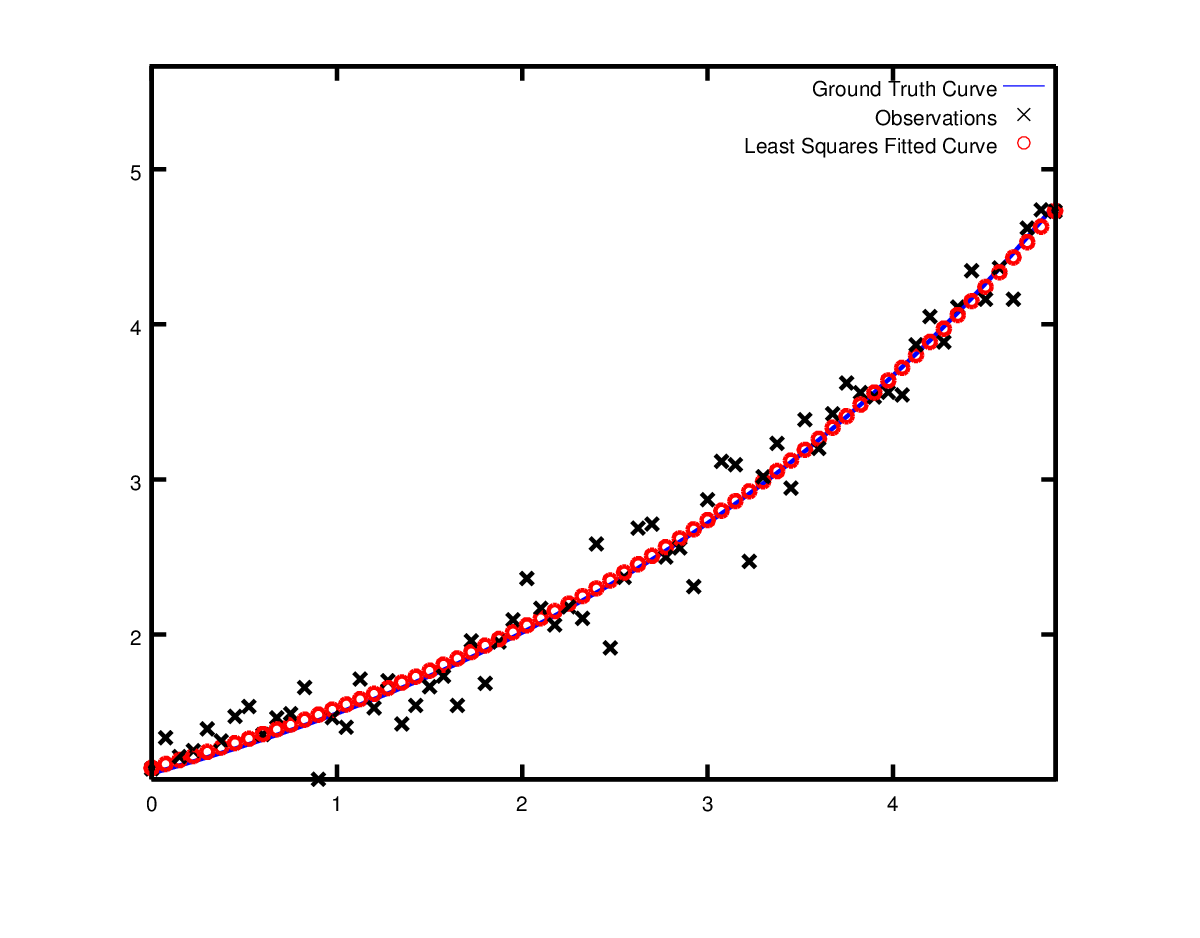
Least squares curve fitting.
Footnotes
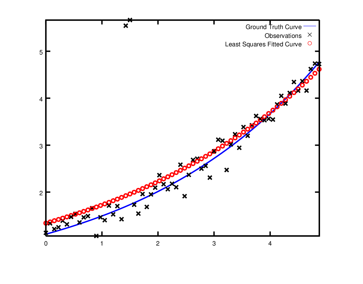
Robust Curve Fitting
Now suppose the data we are given has some outliers, i.e., we have some points that do not obey the noise model. If we were to use the code above to fit such data, we would get a fit that looks as below. Notice how the fitted curve deviates from the ground truth.
To deal with outliers, a standard technique is to use a
LossFunction. Loss functions reduce the influence of
residual blocks with high residuals, usually the ones corresponding to
outliers. To associate a loss function with a residual block, we change
problem.AddResidualBlock(cost_function, nullptr , &m, &c);
to
problem.AddResidualBlock(cost_function, new CauchyLoss(0.5) , &m, &c);
CauchyLoss is one of the loss functions that ships with Ceres
Solver. The argument \(0.5\) specifies the scale of the loss
function. As a result, we get the fit below [7]. Notice how the
fitted curve moves back closer to the ground truth curve.
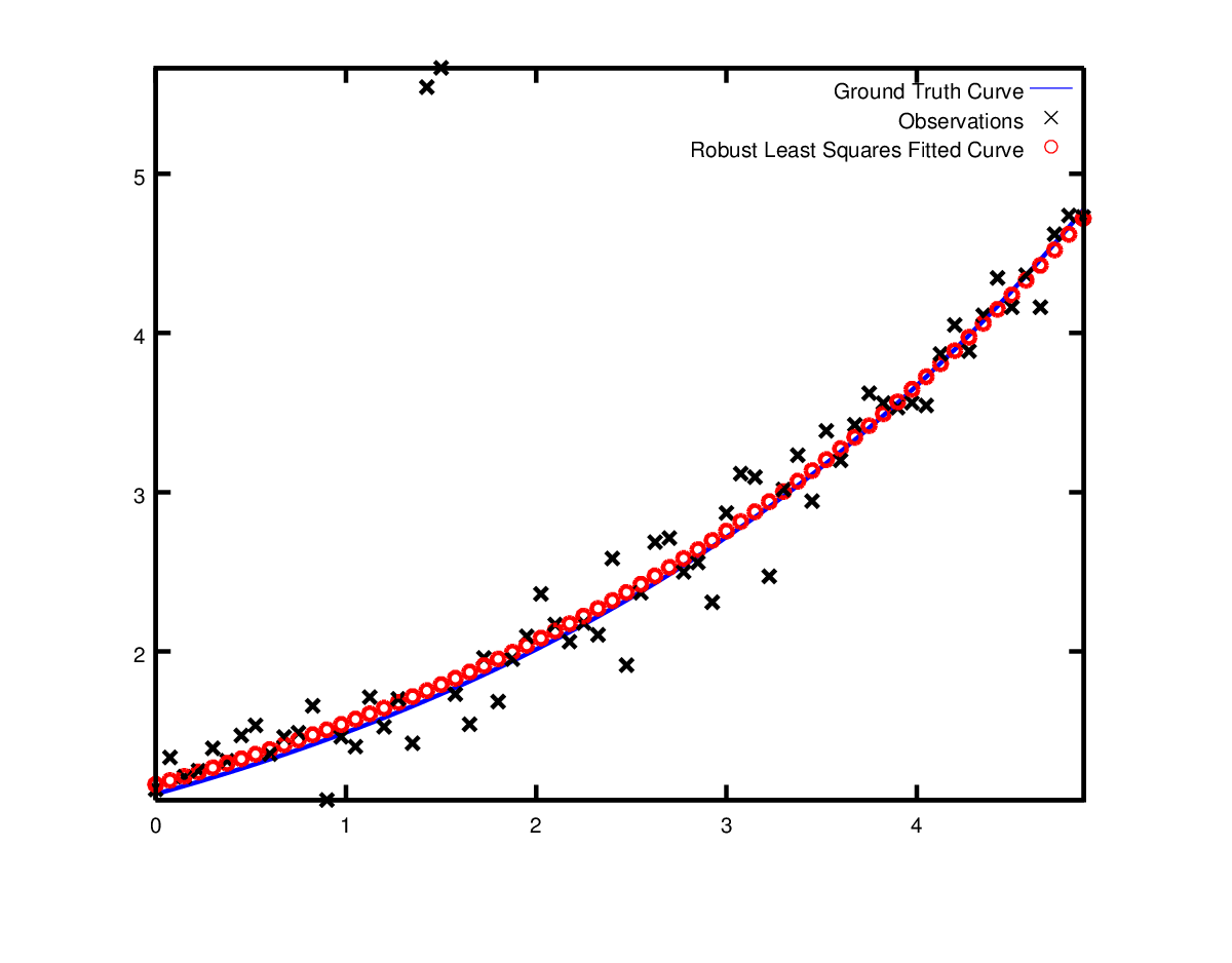
Using LossFunction to reduce the effect of outliers on a
least squares fit.
Footnotes
Bundle Adjustment
One of the main reasons for writing Ceres was our need to solve large scale bundle adjustment problems [HartleyZisserman], [Triggs].
Given a set of measured image feature locations and correspondences, the goal of bundle adjustment is to find 3D point positions and camera parameters that minimize the reprojection error. This optimization problem is usually formulated as a non-linear least squares problem, where the error is the squared \(L_2\) norm of the difference between the observed feature location and the projection of the corresponding 3D point on the image plane of the camera. Ceres has extensive support for solving bundle adjustment problems.
Let us solve a problem from the BAL dataset [8].
The first step as usual is to define a templated functor that computes
the reprojection error/residual. The structure of the functor is
similar to the ExponentialResidual, in that there is an
instance of this object responsible for each image observation.
Each residual in a BAL problem depends on a three dimensional point and a nine parameter camera. The nine parameters defining the camera are: three for rotation as a Rodrigues’ axis-angle vector, three for translation, one for focal length and two for radial distortion. The details of this camera model can be found the Bundler homepage and the BAL homepage.
struct SnavelyReprojectionError {
  SnavelyReprojectionError(double observed_x, double observed_y)
      : observed_x(observed_x), observed_y(observed_y) {}

  template <typename T>
  bool operator()(const T* const camera,
                  const T* const point,
                  T* residuals) const {
    // camera[0,1,2] are the angle-axis rotation.
    T p[3];
    ceres::AngleAxisRotatePoint(camera, point, p);
    // camera[3,4,5] are the translation.
    p[0] += camera[3]; p[1] += camera[4]; p[2] += camera[5];

    // Compute the center of distortion. The sign change comes from
    // the camera model that Noah Snavely's Bundler assumes, whereby
    // the camera coordinate system has a negative z axis.
    T xp = - p[0] / p[2];
    T yp = - p[1] / p[2];

    // Apply second and fourth order radial distortion.
    const T& l1 = camera[7];
    const T& l2 = camera[8];
    T r2 = xp*xp + yp*yp;
    T distortion = 1.0 + r2  * (l1 + l2  * r2);

    // Compute final projected point position.
    const T& focal = camera[6];
    T predicted_x = focal * distortion * xp;
    T predicted_y = focal * distortion * yp;

    // The error is the difference between the predicted and observed position.
    residuals[0] = predicted_x - T(observed_x);
    residuals[1] = predicted_y - T(observed_y);
    return true;
  }

   // Factory to hide the construction of the CostFunction object from
   // the client code.
   static ceres::CostFunction* Create(const double observed_x,
                                      const double observed_y) {
     return new ceres::AutoDiffCostFunction<SnavelyReprojectionError, 2, 9, 3>
       (observed_x, observed_y);
   }

  double observed_x;
  double observed_y;
};
Note that unlike the examples before, this is a non-trivial function
and computing its analytic Jacobian is a bit of a pain. Automatic
differentiation makes life much simpler. The function
AngleAxisRotatePoint() and other functions for manipulating
rotations can be found in include/ceres/rotation.h.
Given this functor, the bundle adjustment problem can be constructed as follows:
ceres::Problem problem;
for (int i = 0; i < bal_problem.num_observations(); ++i) {
  ceres::CostFunction* cost_function =
      SnavelyReprojectionError::Create(
           bal_problem.observations()[2 * i + 0],
           bal_problem.observations()[2 * i + 1]);
  problem.AddResidualBlock(cost_function,
                           nullptr /* squared loss */,
                           bal_problem.mutable_camera_for_observation(i),
                           bal_problem.mutable_point_for_observation(i));
}
Notice that the problem construction for bundle adjustment is very similar to the curve fitting example – one term is added to the objective function per observation.
Since this is a large sparse problem (well large for DENSE_QR
anyways), one way to solve this problem is to set
Solver::Options::linear_solver_type to
SPARSE_NORMAL_CHOLESKY and call Solve(). And while this is
a reasonable thing to do, bundle adjustment problems have a special
sparsity structure that can be exploited to solve them much more
efficiently. Ceres provides three specialized solvers (collectively
known as Schur-based solvers) for this task. The example code uses the
simplest of them DENSE_SCHUR.
ceres::Solver::Options options;
options.linear_solver_type = ceres::DENSE_SCHUR;
options.minimizer_progress_to_stdout = true;
ceres::Solver::Summary summary;
ceres::Solve(options, &problem, &summary);
std::cout << summary.FullReport() << "\n";
For a more sophisticated bundle adjustment example which demonstrates the use of Ceres’ more advanced features including its various linear solvers, robust loss functions and manifolds see examples/bundle_adjuster.cc
Footnotes
Other Examples
Besides the examples in this chapter, the example directory contains a number of other examples:
bundle_adjuster.cc shows how to use the various features of Ceres to solve bundle adjustment problems.
circle_fit.cc shows how to fit data to a circle.
ellipse_approximation.cc fits points randomly distributed on an ellipse with an approximate line segment contour. This is done by jointly optimizing the control points of the line segment contour along with the preimage positions for the data points. The purpose of this example is to show an example use case for
Solver::Options::dynamic_sparsity, and how it can benefit problems which are numerically dense but dynamically sparse.denoising.cc implements image denoising using the Fields of Experts model.
nist.cc implements and attempts to solves the NIST non-linear regression problems.
more_garbow_hillstrom.cc A subset of the test problems from the paper
Testing Unconstrained Optimization Software Jorge J. More, Burton S. Garbow and Kenneth E. Hillstrom ACM Transactions on Mathematical Software, 7(1), pp. 17-41, 1981
which were augmented with bounds and used for testing bounds constrained optimization algorithms by
A Trust Region Approach to Linearly Constrained Optimization David M. Gay Numerical Analysis (Griffiths, D.F., ed.), pp. 72-105 Lecture Notes in Mathematics 1066, Springer Verlag, 1984.
libmv_bundle_adjuster.cc is the bundle adjustment algorithm used by Blender/libmv.
libmv_homography.cc This file demonstrates solving for a homography between two sets of points and using a custom exit criterion by having a callback check for image-space error.
robot_pose_mle.cc This example demonstrates how to use the
DynamicAutoDiffCostFunctionvariant of CostFunction. TheDynamicAutoDiffCostFunctionis meant to be used in cases where the number of parameter blocks or the sizes are not known at compile time.This example simulates a robot traversing down a 1-dimension hallway with noise odometry readings and noisy range readings of the end of the hallway. By fusing the noisy odometry and sensor readings this example demonstrates how to compute the maximum likelihood estimate (MLE) of the robot’s pose at each timestep.
slam/pose_graph_2d/pose_graph_2d.cc The Simultaneous Localization and Mapping (SLAM) problem consists of building a map of an unknown environment while simultaneously localizing against this map. The main difficulty of this problem stems from not having any additional external aiding information such as GPS. SLAM has been considered one of the fundamental challenges of robotics. There are many resources on SLAM [9]. A pose graph optimization problem is one example of a SLAM problem. The following explains how to formulate the pose graph based SLAM problem in 2-Dimensions with relative pose constraints.
Consider a robot moving in a 2-Dimensional plane. The robot has access to a set of sensors such as wheel odometry or a laser range scanner. From these raw measurements, we want to estimate the trajectory of the robot as well as build a map of the environment. In order to reduce the computational complexity of the problem, the pose graph approach abstracts the raw measurements away. Specifically, it creates a graph of nodes which represent the pose of the robot, and edges which represent the relative transformation (delta position and orientation) between the two nodes. The edges are virtual measurements derived from the raw sensor measurements, e.g. by integrating the raw wheel odometry or aligning the laser range scans acquired from the robot. A visualization of the resulting graph is shown below.
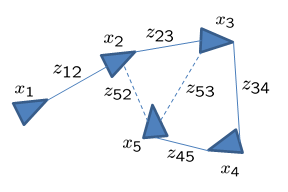
Visual representation of a graph SLAM problem.
The figure depicts the pose of the robot as the triangles, the measurements are indicated by the connecting lines, and the loop closure measurements are shown as dotted lines. Loop closures are measurements between non-sequential robot states and they reduce the accumulation of error over time. The following will describe the mathematical formulation of the pose graph problem.
The robot at timestamp \(t\) has state \(x_t = [p^T, \psi]^T\) where \(p\) is a 2D vector that represents the position in the plane and \(\psi\) is the orientation in radians. The measurement of the relative transform between the robot state at two timestamps \(a\) and \(b\) is given as: \(z_{ab} = [\hat{p}_{ab}^T, \hat{\psi}_{ab}]\). The residual implemented in the Ceres cost function which computes the error between the measurement and the predicted measurement is:
\[\begin{split}r_{ab} = \left[ \begin{array}{c} R_a^T\left(p_b - p_a\right) - \hat{p}_{ab} \\ \mathrm{Normalize}\left(\psi_b - \psi_a - \hat{\psi}_{ab}\right) \end{array} \right]\end{split}\]where the function \(\mathrm{Normalize}()\) normalizes the angle in the range \([-\pi,\pi)\), and \(R\) is the rotation matrix given by
\[\begin{split}R_a = \left[ \begin{array}{cc} \cos \psi_a & -\sin \psi_a \\ \sin \psi_a & \cos \psi_a \\ \end{array} \right]\end{split}\]To finish the cost function, we need to weight the residual by the uncertainty of the measurement. Hence, we pre-multiply the residual by the inverse square root of the covariance matrix for the measurement, i.e. \(\Sigma_{ab}^{-\frac{1}{2}} r_{ab}\) where \(\Sigma_{ab}\) is the covariance.
Lastly, we use a manifold to normalize the orientation in the range \([-\pi,\pi)\). Specially, we define the
AngleManifold::Plus()function to be: \(\mathrm{Normalize}(\psi + \Delta)\) andAngleManifold::Minus()function to be \(\mathrm{Normalize}(y) - \mathrm{Normalize}(x)\).This package includes an executable
pose_graph_2dthat will read a problem definition file. This executable can work with any 2D problem definition that uses the g2o format. It would be relatively straightforward to implement a new reader for a different format such as TORO or others.pose_graph_2dwill print the Ceres solver full summary and then output to disk the original and optimized poses (poses_original.txtandposes_optimized.txt, respectively) of the robot in the following format:pose_id x y yaw_radians pose_id x y yaw_radians pose_id x y yaw_radians
where
pose_idis the corresponding integer ID from the file definition. Note, the file will be sorted in ascending order for thepose_id.The executable
pose_graph_2dexpects the first argument to be the path to the problem definition. To run the executable,/path/to/bin/pose_graph_2d /path/to/dataset/dataset.g2oA python script is provided to visualize the resulting output files.
/path/to/repo/examples/slam/pose_graph_2d/plot_results.py --optimized_poses ./poses_optimized.txt --initial_poses ./poses_original.txt
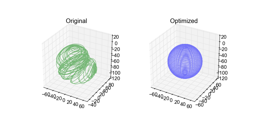
As an example, a standard synthetic benchmark dataset [10] created by Edwin Olson which has 3500 nodes in a grid world with a total of 5598 edges was solved. Visualizing the results with the provided script produces:
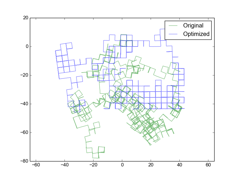
with the original poses in green and the optimized poses in blue. As shown, the optimized poses more closely match the underlying grid world. Note, the left side of the graph has a small yaw drift due to a lack of relative constraints to provide enough information to reconstruct the trajectory.
Footnotes
slam/pose_graph_3d/pose_graph_3d.cc The following explains how to formulate the pose graph based SLAM problem in 3-Dimensions with relative pose constraints. The example also illustrates how to use Eigen’s geometry module with Ceres’s automatic differentiation functionality.
The robot at timestamp \(t\) has state \(x_t = [p^T, q^T]^T\) where \(p\) is a 3D vector that represents the position and \(q\) is the orientation represented as an Eigen quaternion. The measurement of the relative transform between the robot state at two timestamps \(a\) and \(b\) is given as: \(z_{ab} = [\hat{p}_{ab}^T, \hat{q}_{ab}^T]^T\). The residual implemented in the Ceres cost function which computes the error between the measurement and the predicted measurement is:
\[\begin{split}r_{ab} = \left[ \begin{array}{c} R(q_a)^{T} (p_b - p_a) - \hat{p}_{ab} \\ 2.0 \mathrm{vec}\left((q_a^{-1} q_b) \hat{q}_{ab}^{-1}\right) \end{array} \right]\end{split}\]where the function \(\mathrm{vec}()\) returns the vector part of the quaternion, i.e. \([q_x, q_y, q_z]\), and \(R(q)\) is the rotation matrix for the quaternion.
To finish the cost function, we need to weight the residual by the uncertainty of the measurement. Hence, we pre-multiply the residual by the inverse square root of the covariance matrix for the measurement, i.e. \(\Sigma_{ab}^{-\frac{1}{2}} r_{ab}\) where \(\Sigma_{ab}\) is the covariance.
Given that we are using a quaternion to represent the orientation, we need to use a manifold (
EigenQuaternionManifold) to only apply updates orthogonal to the 4-vector defining the quaternion. Eigen’s quaternion uses a different internal memory layout for the elements of the quaternion than what is commonly used. Specifically, Eigen stores the elements in memory as \([x, y, z, w]\) where the real part is last whereas it is typically stored first. Note, when creating an Eigen quaternion through the constructor the elements are accepted in \(w\), \(x\), \(y\), \(z\) order. Since Ceres operates on parameter blocks which are raw double pointers this difference is important and requires a different parameterization.This package includes an executable
pose_graph_3dthat will read a problem definition file. This executable can work with any 3D problem definition that uses the g2o format with quaternions used for the orientation representation. It would be relatively straightforward to implement a new reader for a different format such as TORO or others.pose_graph_3dwill print the Ceres solver full summary and then output to disk the original and optimized poses (poses_original.txtandposes_optimized.txt, respectively) of the robot in the following format:pose_id x y z q_x q_y q_z q_w pose_id x y z q_x q_y q_z q_w pose_id x y z q_x q_y q_z q_w ...
where
pose_idis the corresponding integer ID from the file definition. Note, the file will be sorted in ascending order for thepose_id.The executable
pose_graph_3dexpects the first argument to be the path to the problem definition. The executable can be run via/path/to/bin/pose_graph_3d /path/to/dataset/dataset.g2oA script is provided to visualize the resulting output files. There is also an option to enable equal axes using
--axes_equal/path/to/repo/examples/slam/pose_graph_3d/plot_results.py --optimized_poses ./poses_optimized.txt --initial_poses ./poses_original.txt
As an example, a standard synthetic benchmark dataset [9] where the robot is traveling on the surface of a sphere which has 2500 nodes with a total of 4949 edges was solved. Visualizing the results with the provided script produces: